Introduction to epidermalmorph
introduction-to-epidermalmorph.Rmd
library(dplyr)
library(epidermalmorph)
library(ggplot2)
library(imager)
library(randomcoloR)
library(reshape2)
library(sf)
library(tidyr)
Input for epidermalmorph
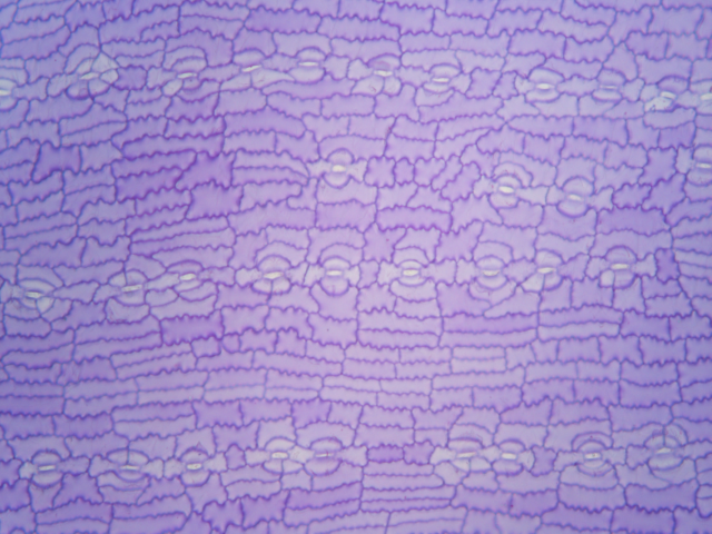
Here is an example of an unprocessed (raw) image of a cuticle preparation cuticle of Podocarpus, taken using a microscope:
For analysis with epidermalmorph, images need to be
segmented (or traced). This can be done manually (e.g. using the paint
tool from ImageJ, MS Paint) or with some degree of automation, but
requires cell wall pixels to be black (value of 0) and no
anti-aliasing to be applied (i.e., the edges of the pixels
should be crisp). Other cell types can be labelled by using different
values (colours). Here is what that might look like:
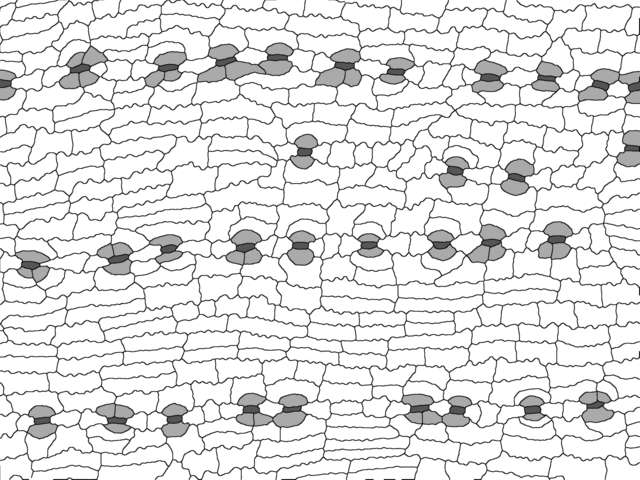
Our cell walls are black (value of 0), stomata are dark grey (85), subsidiary cells are light grey (170) and pavement cells are white (255).
Extracting cell measurements
The image_to_poly() function
Before we can measure cells, they need to be transformed from pixels to polygons:
polys1.1 <- image_to_poly(dir='images', file="traced_im.png")This gives us a list, with an object called cells (our
polygons) and an object called junction_points (used for
cell quantification). We can confirm that this has worked by plotting
our polygons with a unique colour for each cell:
#generate as many random colours as there are cells

n <- nrow(polys1.1$cells)
palette <- distinctColorPalette(n)

ggplot()+
  geom_sf(data=polys1.1$cells, col="black", fill=palette)+
  theme_void()
We can also check that the cell types (as values) have been preserved
during the conversion from pixels to polygons:
We can also check that the cell types (as values) have been preserved
during the conversion from pixels to polygons:
#simplify palette to cell types
palette <- c("#A30B37", "#bd6b73", "#bbb6df")

ggplot()+
  geom_sf(data=polys1.1$cells, col="black", fill=palette[factor(polys1.1$cells$value)])+
  theme_void()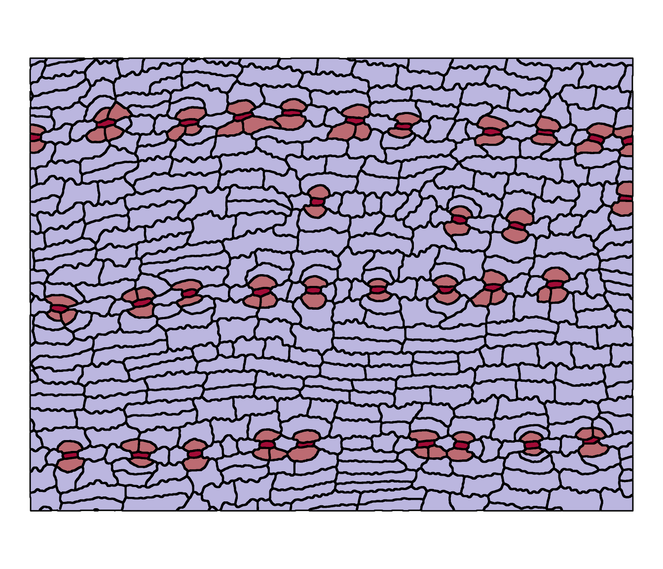
Trait extraction
The stomatal complexes are in red (lighter red shows the subsidiary cells). Now we can extract the measurements from it:
traits1.1 <- extract_epidermal_traits(image.ID = "Image1.1",
                                      cell.polygons=polys1.1$cells,
                                      junction.points=polys1.1$junction_coords,
                                      cells.present = c("pavement", "stomata","subsidiary"),
                                      wall.width = 3,
                                      cell.values=c(255,85, 170),
                                      sd.measures = FALSE, #no variability traits
                                      image.scale = NULL,  verbose=TRUE)
#this can take up to around 10 minutes per image
extract_epidermal_traits returns a list:
-
image_datathe measured traits, summarised to give one value per image -
pavezone_individual_datameasurements for individual pavement zone cells (not adjacent to a stomatal complex) -
stomzone_individual_datameasurements for individual stomatal zone cells (adjacent to a stomatal complex) -
polar_individual_datameasurements for individual polar subsidiary cells (those that share a cell wall with the guard cells/stomatal pore, regardless of whether or not they are considered ‘true’ subsidiary cells) -
stomata_individual_datameasurements for individual stomatal complex -
polygonsthesfpolygons of the cells (removed here to reduce vignette size)
dplyr::glimpse(traits1.1$image_data)
#> Rows: 1
#> Columns: 39
#> $ image.ID                       <chr> "Image1.1"
#> $ rotation                       <dbl> 6.079451
#> $ n.pavement                     <dbl> 340
#> $ n.stomata                      <dbl> 30
#> $ n.subsidiary                   <dbl> 74
#> $ stomatal.density               <dbl> 4.970346e-05
#> $ stomatal.index                 <dbl> 6.326531
#> $ dist.between.stom.rows         <dbl> 236.586
#> $ row.consistency                <dbl> 1
#> $ row.wiggliness                 <dbl> 1.477667
#> $ stom.angle.sd                  <dbl> 0.1616541
#> $ stom.distNN.mean               <dbl> 54.90197
#> $ stom.dist2NN.mean              <dbl> 94.43844
#> $ stom.spacingNN.mean            <dbl> 2.636364
#> $ stom.nsubcells.mean            <dbl> 2.451613
#> $ stom.subsarea.mean             <dbl> 1052.247
#> $ stom.gclength.mean             <dbl> 23.56796
#> $ stom.AR.mean                   <dbl> 1.071619
#> $ stom.butterfly.mean            <dbl> 0.5159461
#> $ stom.symmetry.mean             <dbl> 0.7357696
#> $ pavezone.angle.median          <dbl> -0.05213068
#> $ pavezone.AR.median             <dbl> 2.110892
#> $ pavezone.area.median           <dbl> 1427.611
#> $ pavezone.complexity.median     <dbl> 1.082962
#> $ pavezone.endwallangle.mean     <dbl> 1.497578
#> $ pavezone.endwalldiff.mean      <dbl> 0.302275
#> $ pavezone.njunctionpts.mean     <dbl> 6.025316
#> $ pavezone.undulation.amp.median <dbl> 5.306078
#> $ pavezone.undulation.freq.mean  <dbl> 0.1550792
#> $ stomzone.AR.median             <dbl> 1.715364
#> $ stomzone.area.median           <dbl> 1168.332
#> $ stomzone.complexity.median     <dbl> 1.092794
#> $ stomzone.undulation.amp.median <dbl> 6.878516
#> $ stomzone.undulation.freq.mean  <dbl> 0.1594227
#> $ polar.AR.median                <dbl> 1.293851
#> $ polar.area.median              <dbl> 562.736
#> $ polar.complexity.median        <dbl> 1.06181
#> $ polar.undulation.amp.median    <dbl> 3.906912
#> $ polar.undulation.freq.mean     <dbl> 0.3144654
For a full description of all traits, we can refer to
trait_key:
head(trait_key)
#>          trait   celltype category sd scaledependent
#> 1     image.ID               basic  0              0
#> 2     rotation               basic  0              0
#> 3   n.pavement              number  0              1
#> 4    n.stomata    stomata   number  0              1
#> 5 n.subsidiary subsidiary   number  0              1
#> 6      n.other      other   number  0              1
#>                                                           description
#> 1                                                Identifier for image
#> 2 Rotation of image, either stomatal north or the user input rotation
#> 3                                            Number of pavement cells
#> 4                                                   Number of stomata
#> 5                                          Number of subsidiary cells
#> 6                                               Number of other cells
Which traits can we reliably quantify for a particular group of plants?
In this vignette, we will use nine pre-traced images (three images
per plant, from three plants in the Podocarpaceae) to demonstrate a
possible workflow for epidermalmorph. These cells are from
Acmopyle pancheri (top row), Podocarpus dispermus
(middle row) and Sundacarpus amarus (labeled as Prumnopitys
amara; bottom row). Note that for a family-level study, three
plants would not be sufficient to accurately assess prediction
(see Brown, 2022)
The epidermal cells of these three plants are clearly distinguishable from each other:
load("polys.Rdata")

p <- list()
palette <- c("#A30B37", "#bd6b73", "#bbb6df")

for (i in 1:9){

  p[[i]] <- ggplot()+
          geom_sf(data=polys[[i]]$cells, col="black", fill=palette[factor(polys[[i]]$cells$value)])+
          theme_void()
}

cowplot::plot_grid(plotlist=p, nrow=3)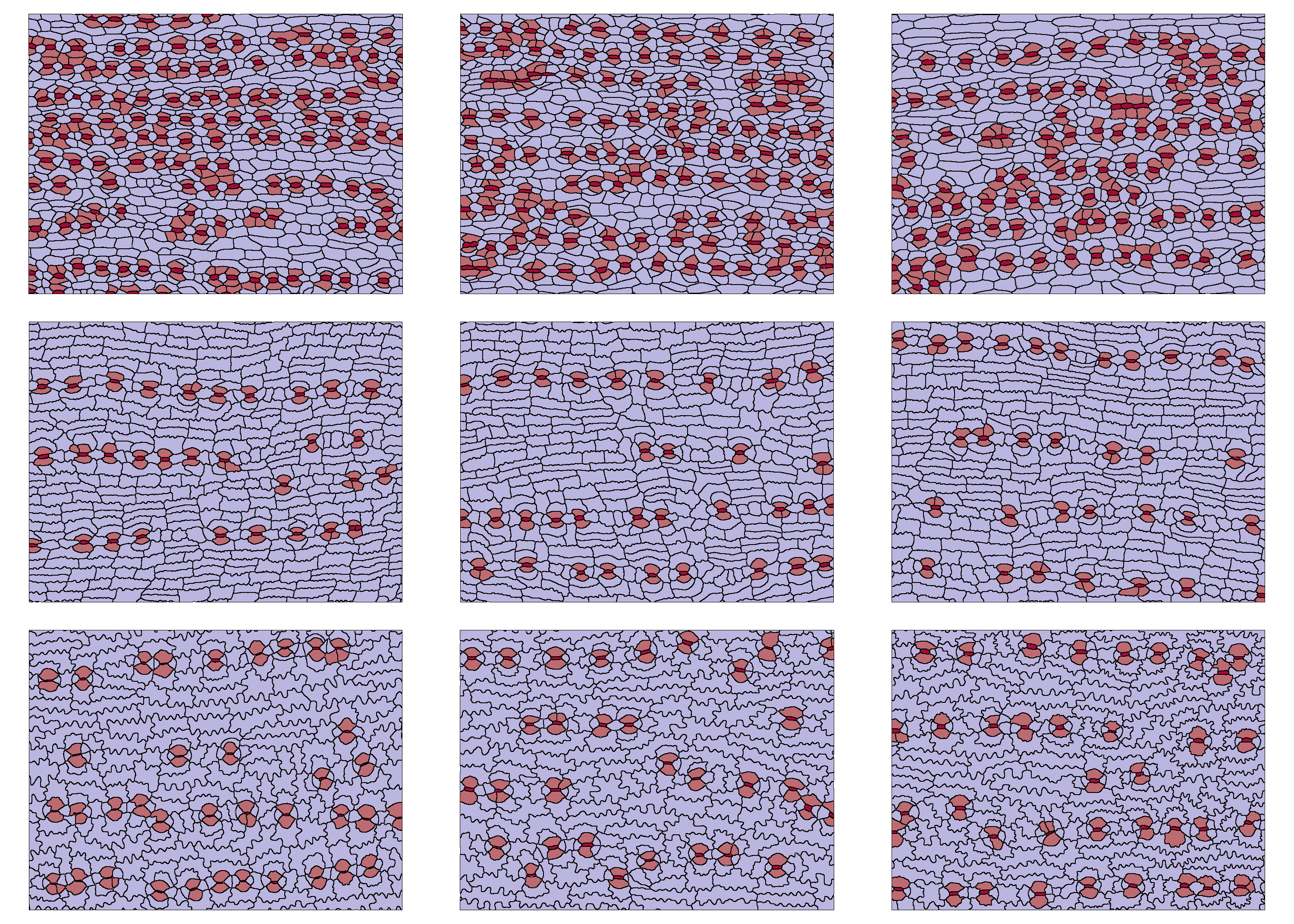
Now we can extract the traits. There is no parallel implementation in
epidermalmorph, but we suggest extracting traits from
multiple images in parallel, like so:
library(parallel)
library(doParallel)
library(foreach)

#names for ID column - the file names of the images
names <- c("Acmopyle_pancheri_1.tif",
           "Acmopyle_pancheri_2.tif",
           "Acmopyle_pancheri_1_3.tif",
           "Podocarpus_dispermus_1.tif",
           "Podocarpus_dispermus_2.tif",
           "Podocarpus_dispermus_3.tif",
           "Sundacarpus_amarus_1.tif",
           "Sundacarpus_amarus_2.tif",
           "Sundacarpus_amarus_3.tif")

cl = makeCluster(3)
registerDoParallel(cl)


df_all <- foreach(i=1:9, .packages = "epidermalmorph") %dopar% {
extract_epidermal_traits(image.ID = names[i],
                         cell.polygons = polys[[i]][[1]],
                         junction.points = polys[[i]][[2]],
                         cells.present = c("pavement", "stomata",
                                           "subsidiary"),
                         sd.measures = FALSE, #no variability traits
                         cell.values=c(255,85,170))
}


stopCluster(cl)
For now, we just want to compare the overall measurements, so we’ll bind the first element of each list together, and scale our trait measurements so that they can be be compared (we’re saving the global standard deviations to be used later):
df_im <- do.call(rbind,lapply(df_all,"[[",1))


globalSDs <- attr(scale(df_im[,10:39]),"scaled:scale") #used later in this vignette

df_im <- df_im %>%
  mutate(across(stomatal.density:polar.undulation.freq.mean,   ~as.numeric(scale(.))))

glimpse(df_im[,1:10]) #only show first 10 columns for brevity
#> Rows: 9
#> Columns: 10
#> $ image.ID               <chr> "Acmopyle_pancheri_1_1.tif", "Acmopyle_pancheri…
#> $ rotation               <dbl> -1.6433946, -5.6864687, 0.4205948, -1.2037529, …
#> $ n.pavement             <dbl> 586, 577, 485, 359, 357, 352, 260, 246, 268
#> $ n.stomata              <dbl> 120, 116, 96, 31, 30, 31, 36, 30, 36
#> $ n.subsidiary           <dbl> 259, 286, 205, 67, 67, 67, 76, 64, 73
#> $ stomatal.density       <dbl> 1.6138089, 1.3029417, 1.0369279, -0.6485418, -0…
#> $ stomatal.index         <dbl> 1.33648596, 1.08367330, 1.26368431, -1.04454500…
#> $ dist.between.stom.rows <dbl> -0.9696199, -1.2562436, -0.9510668, 1.3375655, …
#> $ row.consistency        <dbl> 1.06181364, 1.35092871, 0.74826970, 0.69230347,…
#> $ row.wiggliness         <dbl> -0.16892056, 1.89337838, 0.30717709, -0.2887358…
This data is only identified by the image filename - we need to add the image metadata (here, with species and individual information)
df_meta <- read.csv("example_metadata.csv", fileEncoding = 'UTF-8-BOM')

glimpse(df_meta)
#> Rows: 9
#> Columns: 5
#> $ image.ID   <chr> "Acmopyle_pancheri_1_1.tif", "Acmopyle_pancheri_1_2.tif", "…
#> $ Genus      <chr> "Acmopyle", "Acmopyle", "Acmopyle", "Podocarpus", "Podocarp…
#> $ species    <chr> "pancheri", "pancheri", "pancheri", "dispermus", "dispermus…
#> $ taxon      <chr> "Acmopyle_pancheri", "Acmopyle_pancheri", "Acmopyle_pancher…
#> $ individual <chr> "Acmopyle_pancheri1", "Acmopyle_pancheri1", "Acmopyle_panch…

df_im <- left_join(df_meta, df_im)
#> Joining, by = "image.ID"
Now we can look at how much intra-individual variation there is in each of our measured traits.
One way we can visualise this is by plotting each measurement for each individual, where larger ranges (wider bars) indicate less intra-individual variation:
df_im_long <- df_im %>%
pivot_longer(10:43)
ggplot(df_im_long)+
geom_point(aes(x=name, y=value, group=individual, col=individual))+
geom_line(aes(x=name, y=value, group=name, col=individual))+
theme(axis.text.x = element_blank(),
axis.text.y = element_blank())+
facet_wrap(vars(individual))+
coord_flip()+
ggpubr::theme_pubclean()+
theme(legend.position = "bottom",legend.direction="vertical")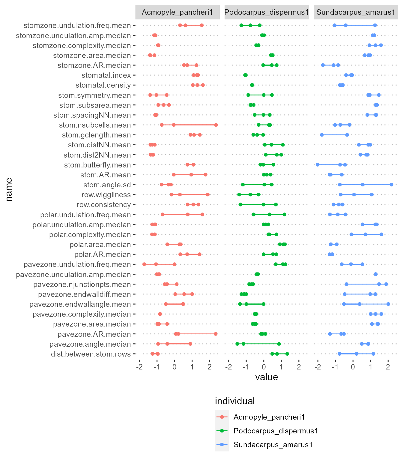 This is an intuitive way to look at trait reliability, but gets out of
hand quickly when considering a larger set of individuals/species.
This is an intuitive way to look at trait reliability, but gets out of
hand quickly when considering a larger set of individuals/species.
epidermalmorph includes the
epidermal_trait_reliability function, which produces a list
of two objects:
- a data.frame with the reliability estimates
- a ggplot heatmap visualisation of this information, where the colour of the tile represents the width of the corresponding line in the above plot
df_reliability <- epidermal_trait_reliability(df_im,
                                              grouping.variable="individual",
                                              heatmap = TRUE)
df_reliability[[2]]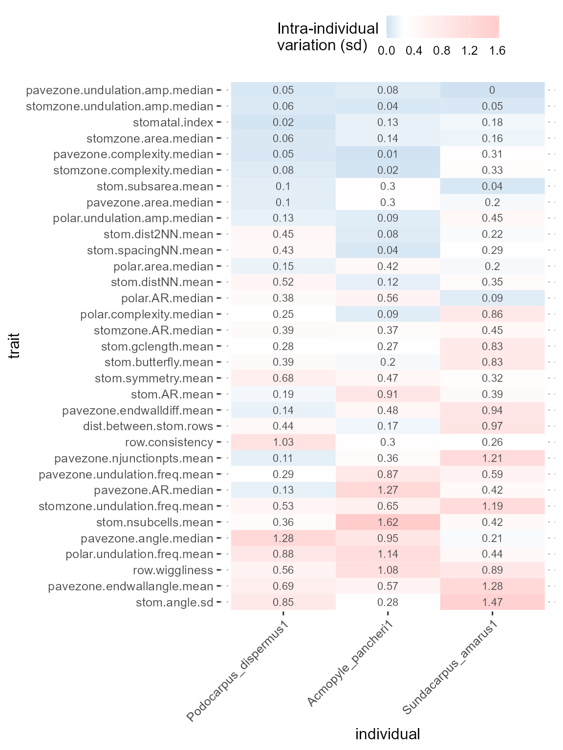
From this, it is easier to see that Podocarpus dispermus
tends to be more consistent across images, and if we define a reliable
trait as one that has a within-individual variation of no more than 25%
of the total variation (i.e. thresholdval = 0.25), we can
identify four traits that can be reliably measured from an image of each
of these plants: stomzone.area.median, stomatal.index,
stomzone.undulation.amp.median, pavezone.undulation.amp.median
Note that for this set of podocarps, stomatal index is one of the most reliable traits that can be measured from an image - this is not the case when analysing a wider set of plants (Brown, 2022), highlighting the need to calibrate these measurements carefully to the study system and select a representative subset of this group to evaluate reliability.
We can extract these traits automatically using the data.frame that
is returned by epidermal_trait_reliability() - here is one
example of how that could be done:
How many cells do I need to trace?
The limiting step in the epidermalmorph workflow is
undoubtedly the segmentation, or tracing of images, so it is useful to
know how many cells we need to measure to get a good estimate of the
traits for that individual or species.
epidermalmorph provides a function to do this. By
repeatedly subsampling patches of cells (i.e. simulating tracing only a
portion of an image) then plotting how much the measured traits differ
from the groundtruth (the trait value measured from all cells in an
image). For more details, see Brown (2022).
This should be done for the same imageset that is used to evaluate trait reliability, but for demonstration purposes, here we will only use Image1.1 (from above).
Here, we repeat trait measurements using small patches of cells from the image. As noted above, we do not include parallel execution in the package but suggest that this step could be run in parallel for multiple images:
df <- subsample_epidermal_traits(traits1.1, n.runs = 100,
                                 k.cells = c(15,50,100,150,200,250,300,350,400),
                                 scaling =globalSDs,
                                 trait.subset = reliable_traits)
If we were analysing multiple images, we would then bind the rows for each image into one data.frame (we have kept these two functions separate to facilitate parallel execution).
Then, we can evaluate how each trait measurement varies over different sample sizes by plotting the standard deviation of sampled measurements against the number of relevant cells (see Brown, 2022 for details).
Points in the grey represent trait-sample combinations that are above the user-defined threshold (here, 20% of the global variation)
p <- subsampling_summary(df, traits=reliable_traits, thresholdvalue = 0.2, number.of.bins = 8)
cowplot::plot_grid(plotlist=p[[1]], ncol=1,align = "v")
#> Warning: Removed 4 rows containing missing values (geom_point).
#> Warning: Removed 4 row(s) containing missing values (geom_path).
#> Warning: Removed 3 rows containing missing values (geom_point).
#> Warning: Removed 3 row(s) containing missing values (geom_path).
#> Warning: Removed 1 rows containing missing values (geom_point).
#> Warning: Removed 1 row(s) containing missing values (geom_path).
#> Warning: Removed 1 rows containing missing values (geom_point).
#> Warning: Removed 1 row(s) containing missing values (geom_path).
#> Warning: Removed 2 rows containing missing values (geom_point).
#> Warning: Removed 2 row(s) containing missing values (geom_path).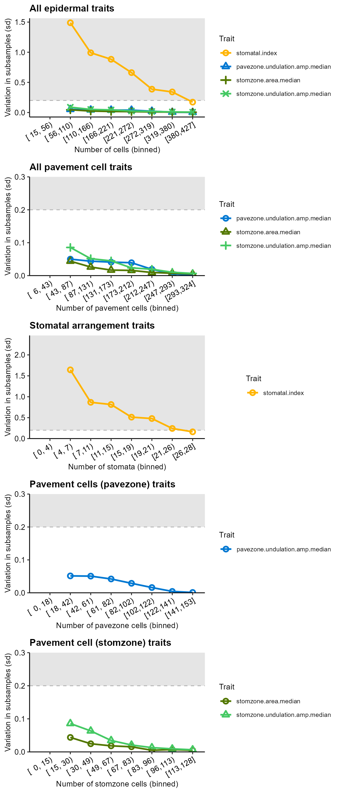
From these plots, we can see that, for this image:
- 100 cells in total is sufficient for pavement cell traits to be measured
- 50 pavement cells in total is sufficient for pavement cell traits (from all zones)
- 30 stomata (or more) are required to measure stomatal index
- For specific types of pavement cells (pavezone, stomzone), 20-40 cells are sufficient.
We recommend that analyses of trait reliability and sampling effort
be done for any study that employs epidermalmorph to
provide evidence that trait measurements and cell sample sizes are
sufficient to reliably measure traits.